A Proof of Brill’s Theorem via Directional Derivatives

Let $K$ be the field of real numbers $\mathbb{R}$ or the field of complex numbers $\mathbb{C}$ . Given a vector $v = (v_1, \ldots, v_n) \in K^n$ . The directional derivative operator with respect to the vector $v$ , denoted by $D_v$ , is a map from the ring $K[x_1, \ldots, x_n]$ to itself, defined by

$\displaystyle D_v(P) = \sum_{i=1}^n v_i \frac{\partial P}{\partial x_i},$

where $\frac{\partial P}{\partial x_i}$ is the formal partial derivative of the polynomial $P$ with respect to the variable $x_i$ .

Theorem 1. Let $P, Q \in K[x_1, \ldots, x_n]$ , constants $a, b \in K$ , and a linear form $L(x) = c_1x_1 + \ldots + c_nx_n$ . The operator $D_v$ has the following properties.

(1) $D_v(aP + bQ) = aD_v(P) + bD_v(Q)$ .

(2) $D_v(PQ) = D_v(P)Q + P D_v(Q)$ .

(3) For any positive integer $k$ , $D_v(P^k) = k P^{k-1} D_v(P)$ .

(4) $D_v(L) = L(v)$ .

Proof. (1) By the definition of the partial derivative of a polynomial, we have

$\displaystyle \frac{\partial (aP + bQ)}{\partial x_i} = a\frac{\partial P}{\partial x_i} + b\frac{\partial Q}{\partial x_i},$

thus we immediately obtain $\displaystyle D_v(aP + bQ) = aD_v(P) + bD_v(Q).$

(2) Since the formal partial derivative obeys the product rule

$\displaystyle \frac{\partial (PQ)}{\partial x_i} = \frac{\partial P}{\partial x_i}Q + P\frac{\partial Q}{\partial x_i}$ we have

$\displaystyle D_v(PQ) = \sum_{i=1}^n v_i \left( \frac{\partial P}{\partial x_i}Q + P\frac{\partial Q}{\partial x_i} \right)$

$\displaystyle = \left( \sum_{i=1}^n v_i \frac{\partial P}{\partial x_i} \right) Q + P \left( \sum_{i=1}^n v_i \frac{\partial Q}{\partial x_i} \right) = D_v(P)Q + P D_v(Q).$

(3) We prove this by mathematical induction on $k$ .

For $k=1$ , the formula becomes $D_v(P^1) = 1 \cdot P^0 \cdot D_v(P)$ , which is trivially true.

Suppose the property holds for $k-1$ , that is

$\displaystyle D_v(P^{k-1}) = (k-1)P^{k-2}D_v(P).$

Applying (2), we obtain

$\displaystyle D_v(P^k) = D_v(P)P^{k-1} + P D_v(P^{k-1})$

$=D_v(P)P^{k-1} + P \big( (k-1)P^{k-2}D_v(P) \big)=k P^{k-1} D_v(P).$

By the principle of mathematical induction, the property holds for all positive integers $k$ .

(4) For a linear form $L(x) = c_1x_1 + \ldots + c_nx_n$ , we have

$\displaystyle D_v(L) = \sum_{i=1}^n v_i \frac{\partial L}{\partial x_i} = \sum_{i=1}^n v_i c_i = L(v).$

The theorem is completely proved. $\Box$

Theorem 2 (Brill). Suppose $K$ is the field of real numbers $\mathbb{R}$ or the field of complex numbers $\mathbb{C}$ . Let $L_1, L_2, \ldots, L_m$ be $m$ non-zero linear forms in $n$ $(n>1)$ variables that are pairwise non-proportional over $K$ . Then, for any integer $k \ge m-1$ , the set of powers $\{L_1^k, L_2^k, \ldots, L_m^k\}$ is linearly independent over $K$ .

Proof. We prove the theorem by mathematical induction on the number of linear forms $m$ . For $m=1$ , we have 1 non-zero linear form $L_1$ . For any integer $k \ge 0$ , the polynomial $L_1^k$ is not the zero polynomial, so the set consisting of only one element $\{L_1^k\}$ is trivially linearly independent. Thus, the assertion holds for $m=1$ .

Now suppose the assertion holds for $m-1$ linear forms, for some integer $m > 1$ . Consider $m$ non-zero pairwise non-proportional linear forms $L_1, \ldots, L_m$ and an exponent $k \ge m-1$ .

Consider the linear relation

$\displaystyle \sum_{i=1}^m c_i L_i^k = 0$ (1)

where $c_i \in K$ . We need to show that $c_i = 0$ for all $i = 1, \ldots, m$ .

Since $L_m$ is not identically $0$ , the set of points $x \in K^n$ such that $L_m(x) = 0$ is an $(n-1)$ -dimensional vector subspace of the space $K^n$ . At the same time, since $L_i$ is not proportional to $L_m$ for all $i < m$ , the intersection of the two spaces $L_i(x) = 0$ and $L_m(x) = 0$ is an $(n-2)$ -dimensional subspace.

The field $K$ has characteristic $0$ and is therefore an infinite field. A vector space over an infinite field cannot be the union of finitely many proper subspaces (see [1]). Therefore, there exists a vector $v = (v_1, \ldots, v_n) \in K^n$ such that $L_m(v) = 0$ and $\displaystyle L_i(v) \neq 0, \quad \forall i = 1, \ldots, m-1.$

Consider the directional derivative operator with respect to the vector $v$ defined as follows

$\displaystyle D_v = \sum_{j=1}^n v_j \frac{\partial}{\partial x_j}.$

When applying $D_v$ to a linear form $\displaystyle L(x) = a_1x_1 + \ldots + a_nx_n,$

we have $\displaystyle D_v(L) = a_1v_1 + \ldots + a_nv_n = L(v).$

When applying this operator to the $k$ -th power of $L$ , we obtain

$\displaystyle D_v(L^k) = k \cdot L^{k-1} \cdot D_v(L) = k \cdot L(v) \cdot L^{k-1}.$

Applying the operator $D_v$ to both sides of equation (1), we have

$\displaystyle \sum_{i=1}^m c_i k L_i(v) L_i^{k-1} = 0.$

Since $L_m(v) = 0$ , the $m$ -th term vanishes completely. Since $m \ge 2$ , we have $k \ge m-1 \ge 1$ , so we can divide both sides by $k$ (which is valid since $K$ has characteristic $0$ ) to obtain

$\displaystyle \sum_{i=1}^{m-1} \big(c_i L_i(v)\big) L_i^{k-1} = 0.$

Since $k \ge m-1$ , we deduce that $k-1 \ge m-2$ . Applying the inductive hypothesis to $m-1$ linear forms with the exponent $k-1$ , the set of polynomials $\{L_1^{k-1}, \ldots, L_{m-1}^{k-1}\}$ is linearly independent. Therefore, all coefficients in the sum above must be zero. That is,

$\displaystyle c_i L_i(v) = 0, \quad \forall i = 1, \ldots, m-1.$ But by the choice of the vector $v$ , we already have $L_i(v) \neq 0$ , so we must have $\displaystyle c_i = 0, \quad \forall i = 1, \ldots, m-1.$ Substituting $c_1 = \ldots = c_{m-1} = 0$ back into (1), we have $c_m L_m^k = 0$ . Since $L_m$ is not zero, $c_m = 0$ .

Thus $c_1 = c_2 = \ldots = c_m = 0$ , and $\{L_1^k, L_2^k, \ldots, L_m^k\}$ is linearly independent. By the principle of mathematical induction, the theorem is proved. $\Box$

References

[1] https://nttuan.org/2010/02/04/finite-unions-of-proper-subspaces-over-an-infinite-field/

The Motzkin-Straus Theorem

To fully comprehend this topic, a basic understanding of multivariable calculus is required. A highly recommended reference is [1], specifically Theorem 2.4.15.

Let $\displaystyle G$ be a simple, undirected graph with vertices labeled as $\displaystyle 1, 2, \dots, n$ . Let $\displaystyle S$ be the set of all non-negative real vectors whose components sum to $\displaystyle 1$ :

$\displaystyle S = \left\{ x = (x_1, x_2, \dots, x_n) \in \mathbb{R}^n \;\middle|\; x_i \ge 0 \text{ for all } i=1,\dots,n, \text{ and } \sum_{i=1}^{n} x_i = 1 \right\}.$

For any vector $\displaystyle x \in S$ , we define the objective function $\displaystyle f(x)$ as the sum of the products of the weights associated with adjacent vertices in $\displaystyle G$ :

$\displaystyle f(x) = \sum_{(i,j) \in E} x_i x_j. \qquad (1)$

Here, each edge $\displaystyle (i,j) = (j,i) \in E$ is counted exactly once. The Motzkin-Straus theorem investigates the maximum value of this function over the set $\displaystyle S$ , denoted as:

$\displaystyle f(G) = \max_{x \in S} f(x) = \max_{x \in S} \sum_{(i,j) \in E} x_i x_j.$

Remark on Existence: The function $\displaystyle f(x)$ defined in (1) is a polynomial, which implies it is continuous everywhere on $\displaystyle \mathbb{R}^n$ . Furthermore, the domain $\displaystyle S$ is a closed and bounded set (a compact set) in $\displaystyle \mathbb{R}^n$ . According to the Extreme Value Theorem, any continuous real-valued function attains both a global maximum and a global minimum on a closed and bounded domain. Therefore, the maximum value $\displaystyle f(G)$ is strictly guaranteed to exist.

Theorem (Motzkin-Straus, 1965). Let $\displaystyle k$ be the clique number (the order of the largest complete subgraph) of $\displaystyle G$ . Then

$\displaystyle f(G)=\frac{1}{2}\left(1-\frac{1}{k}\right). \qquad (2)$

Proof. Suppose $\displaystyle x = (x_1, x_2, \dots, x_n)$ is a point in $\displaystyle S$ that maximizes the function

$\displaystyle f(x) = \sum_{(i,j)\in G} x_i x_j.$

Let $\displaystyle V_x = \{i \mid x_i > 0\}$ be the set of vertices with positive weights. Suppose $\displaystyle V_x$ does not induce a complete subgraph (clique). Then, there exist at least two vertices $\displaystyle u, v \in V_x$ that are not adjacent in $\displaystyle G$ .

Let $\displaystyle S_u = \sum_{j \in N(u)} x_j$ and $\displaystyle S_v = \sum_{j \in N(v)} x_j$ be the sum of the weights of the neighbors of $\displaystyle u$ and $\displaystyle v$ in $\displaystyle G$ , respectively. Without loss of generality, assume that $\displaystyle S_u \le S_v$ .

We construct a new weight distribution $\displaystyle x'$ by shifting the entire weight of $\displaystyle u$ to $\displaystyle v$ :

$\displaystyle x'_u = 0$
$\displaystyle x'_v = x_u + x_v$
$\displaystyle x'_i = x_i$ for all $\displaystyle i \neq u, v$ .

It is clear that $\displaystyle x' \in S$ because the total weight remains $\displaystyle 1$ and all weights remain non-negative. The change in the objective function is given by

$\displaystyle f(x') - f(x) = x_u (S_v - S_u).$

Since $\displaystyle x_u > 0$ and $\displaystyle S_v \ge S_u$ , we have $\displaystyle f(x') \ge f(x)$ . However, because $\displaystyle x$ is already a global maximizer, it must hold that $\displaystyle f(x') = f(x)$ .

The new point $\displaystyle x'$ still achieves the maximum value, but the number of vertices with positive weights has decreased by 1 (since $\displaystyle x'_u = 0$ ). We repeat this weight-shifting process for any remaining pair of non-adjacent vertices with positive weights. This process must terminate after a finite number of steps. Upon termination, all vertices with positive weights must be mutually adjacent, meaning they form a complete subgraph $\displaystyle C$ .

Let $\displaystyle m$ be the number of vertices in $\displaystyle C$ . Since $\displaystyle k$ is the clique number of $\displaystyle G$ , we must have $\displaystyle m \le k$ . On the complete subgraph $\displaystyle C$ , all vertices are pairwise adjacent, so

$\displaystyle f(x) = \sum_{(i,j) \in C} x_i x_j = \frac{1}{2} \left( \left( \sum_{i \in C} x_i \right)^2 - \sum_{i \in C} x_i^2 \right).$

Since the sum of the weights on $\displaystyle C$ is $\displaystyle \sum_{i \in C} x_i = 1$ , we obtain

$\displaystyle f(x) = \frac{1}{2} \left( 1 - \sum_{i \in C} x_i^2 \right).$

By the Cauchy-Schwarz inequality, we have

$\displaystyle \sum_{i \in C} x_i^2 \ge \frac{1}{m} \left( \sum_{i \in C} x_i \right)^2 = \frac{1}{m}.$

This implies $\displaystyle f(x) \le \frac{1}{2} \left( 1 - \frac{1}{m} \right).$

Since the function $\displaystyle g(m) = \frac{1}{2}\left(1 - \frac{1}{m}\right)$ is strictly increasing with respect to $\displaystyle m$ and $\displaystyle m \le k$ , we get:

$\displaystyle f(x) \le \frac{1}{2} \left( 1 - \frac{1}{k} \right). \qquad (3)$

Now, choose a maximum complete subgraph of $\displaystyle G$ with order $\displaystyle k$ . Assume the vertices of this subgraph are $\displaystyle 1, 2, \dots, k$ . By distributing the total weight equally among these $\displaystyle k$ vertices and setting the weights of all other vertices to $\displaystyle 0$ , i.e.,

$\displaystyle x_1 = x_2 = \dots = x_k = \frac{1}{k} \quad \text{and} \quad x_{k+1} = \dots = x_{n} = 0,$

we can compute the value of the objective function at this specific point as:

$\displaystyle f(x) = \binom{k}{2} \cdot \frac{1}{k^2} = \frac{k(k-1)}{2} \cdot \frac{1}{k^2} = \frac{1}{2} \left( 1 - \frac{1}{k} \right). \qquad (4)$

Combining (3) and (4), we conclude that the maximum value of the objective function on the set $\displaystyle S$ is precisely $\displaystyle f(G) = \frac{1}{2}\left(1 - \frac{1}{k}\right).$

This completes the proof. ∎

Corollary (Turán’s Theorem). Let $\displaystyle G$ be a graph with $\displaystyle n$ vertices and edge set $\displaystyle E$ . If $\displaystyle G$ contains no complete subgraph of order $\displaystyle k+1$ (meaning the clique number of $\displaystyle G$ does not exceed $\displaystyle k$ ), then the number of edges in $\displaystyle G$ satisfies

$\displaystyle |E| \le \frac{n^2}{2} \left( 1 - \frac{1}{k} \right).$

Proof. Consider the uniform weight distribution $\displaystyle x = \left(\frac{1}{n}, \frac{1}{n}, \dots, \frac{1}{n}\right)$ . Clearly, $\displaystyle x \in S$ since all coordinates are non-negative and their sum equals 1.

Evaluating the objective function $\displaystyle f(x)$ at this point, each edge $\displaystyle (i,j) \in G$ contributes exactly $\displaystyle \frac{1}{n} \cdot \frac{1}{n} = \frac{1}{n^2}$ . Since the graph $\displaystyle G$ has $\displaystyle |E|$ edges, we have:

$\displaystyle f(x) = \sum_{(i,j) \in G} x_i x_j = \sum_{(i,j) \in G} \frac{1}{n^2} = \frac{|E|}{n^2}.$

On the other hand, by the Motzkin-Straus Theorem, the value of $\displaystyle f(x)$ at any point in $\displaystyle S$ cannot exceed the global maximum $\displaystyle f(G)$ . Let $\displaystyle m$ be the clique number of $\displaystyle G$ . By hypothesis, $\displaystyle m \le k$ . Therefore:

$\displaystyle f(x) \le f(G) = \frac{1}{2} \left( 1 - \frac{1}{m} \right) \le \frac{1}{2} \left( 1 - \frac{1}{k} \right).$

Combining these two results, we obtain $\displaystyle |E| \le \frac{n^2}{2} \left( 1 - \frac{1}{k} \right).$

The inequality is thus proven. ∎

References
[1] Jerry Shurman, Calculus and Analysis in Euclidean Space (pages 23-56).

Formal power series

Định nghĩa 1. Một chuỗi lũy thừa hình thức là một biểu diễn có dạng

$a_0+a_1x+a_2x^2+a_3x^3+\ldots,$

hay gọn hơn $\displaystyle\sum_{k=0}^{\infty}a_kx^k.$ Trong đó $(a_n)_{n\geq 0}$ là một dãy các số phức. Các $a_i$ được gọi là các hệ số của chuỗi lũy thừa hình thức, $a_0$ được gọi là hệ số tự do của chuỗi lũy thừa hình thức.

Từ “hình thức” trong định nghĩa trên có nghĩa là ta không bận tâm đến việc cho $x$ các giá trị đặc biệt, ta cũng không quan tâm đến tính hội tụ hay phân kỳ của chuỗi. Tập tất cả các chuỗi lũy thừa hình thức với hệ số thuộc một tập hợp $A$ được ký hiệu bởi $A[[x]]$ . Với một chuỗi lũy thừa hình thức $a(x)$ , ta ký hiệu hệ số của $x^n$ trong chuỗi này bởi $[x^n]a(x)$ .

Nếu $a_i=0$ với mọi $i>m$ thì để cho gọn, chuỗi $\sum_{n=0}^{\infty}a_nx^n$ sẽ được viết là

$a_0+a_1x+\ldots+a_mx^m.$

Chuỗi lũy thừa hình thức với tất cả các hệ số bằng $0$ được gọi là chuỗi không, ký hiệu là $0$ . Tổng và tích của hai chuỗi lũy thừa hình thức $\displaystyle\sum_{n=0}^{\infty}a_nx^n$ và $\displaystyle\sum_{n=0}^{\infty}b_nx^n$ được định nghĩa bởi

$\displaystyle\sum_{n=0}^{\infty}a_nx^n+\sum_{n=0}^{\infty}b_nx^n=\sum_{n=0}^{\infty}(a_n+b_n)x^n$

và

$\displaystyle\left(\sum_{n=0}^{\infty}a_nx^n\right)\left(\sum_{n=0}^{\infty}b_nx^n\right)=\sum_{n=0}^{\infty}\left(\sum_{k=0}^na_kb_{n-k}\right)x^n.$

Với hai phép toán này thì $\mathbb{C}[[x]]$ là một vành giao hoán có đơn vị là chuỗi đơn vị $1+0x^1+0x^2+0x^3+\ldots,$ ký hiệu là $1$ .

Tương tự như với các số phức, ta có kết quả sau:

Định lý 1. Nếu $a$ và $b$ là các phần tử khác không của $\mathbb{C}[[x]]$ , thì chuỗi tích $ab$ cũng khác chuỗi không.

Chứng minh. Gọi $m$ là số tự nhiên nhỏ nhất sao cho $[x^m]a\not=0$ , và $n$ là số tự nhiên nhỏ nhất sao cho $[x^n]b\not=0$ . Khi đó

$[x^{m+n}](ab)=([x^m]a)([x^n]b)\not=0,$

suy ra $ab$ khác chuỗi không. $\Box$

Khác với phép nhân trong tập các số phức, không phải mọi chuỗi khác không đều có nghịch đảo. Chẳng hạn, khi $a(x)=0+x+0x^2+0x^3+\ldots,$ (chuỗi này thường được viết là $a(x)=x$ ) thì $a(x)\not=0$ nhưng không có chuỗi $b(x)$ để $a(x)b(x)=1$ .

Định lý 2. Chuỗi $a(x)$ có nghịch đảo khi và chỉ khi $[x^0]a(x)\not=0$ .

Chứng minh. Giả sử chuỗi $a(x)$ có nghịch đảo, và $b(x)$ là nghịch đảo của nó. Khi đó

$1=[x^0](ab)=([x^0]a)([x^0]b),$

suy ra $[x^0]a(x)\not=0$ .

Bây giờ giả sử $\displaystyle a(x)=\sum_{n=0}^{\infty}a_nx^n$ là một chuỗi lũy thừa hình thức có $a_0=[x^0]a(x)\not=0$ . Chuỗi lũy thừa hình thức $\displaystyle b(x)=\sum_{n=0}^{\infty}b_nx^n$ là nghịch đảo của $a(x)$ khi và chỉ khi $a_0b_0=1$ và

$\displaystyle\sum _{k=0}^na_kb_{n-k}=0,\quad\forall n\geq 1.$

Từ hệ này ta có thể xác định $b(x)$ bởi $b_0=1/a_0$ và

$\displaystyle b_n=-\frac{1}{a_0}\sum _{k=1}^na_kb_{n-k},\quad\forall n\geq 1.$ $\Box$

Khi $a$ là một chuỗi có nghịch đảo thì ta ký hiệu chuỗi nghịch đảo của nó bởi $a^{-1}$ . Tích của chuỗi $b$ và chuỗi $a^{-1}$ thường được viết là $\frac{b}{a}$ .

Ví dụ. Chuỗi lũy thừa hình thức $1-x$ có nghịch đảo là chuỗi

$\displaystyle \frac{1}{1-x}=1+x+x^2+x^3+\ldots$

Định nghĩa 2. Dãy các chuỗi lũy thừa hình thức với hệ số phức $\{S_n(x)\}_{n\geq 1}$ được gọi là hội tụ đến chuỗi lũy thừa hình thức với hệ số phức $S(x)$ , ký hiệu $\displaystyle\lim_{n\to\infty} S_n(x)=S(x)$ , nếu với mỗi $n\geq 0$ có số nguyên dương $N$ sao cho $[x^n]S_i(x)=[x^n]S(x)$ mỗi khi $i\geq N$ . Trong trường hợp này ta nói $\{S_n(x)\}_{n\geq 1}$ là một dãy hội tụ.

Khi $\displaystyle A(x)=\sum_{n\geq 0}a_nx^n$ là một phần tử khác không của $\mathbb{C}[[x]]$ , ta gọi bậc của $A(x)$ , ký hiệu $\deg A(x)$ , là số $n$ nhỏ nhất sao cho $a_n\not=0$ . Dễ thấy nếu $B(x)$ và $C(x)$ là các phần tử khác không của $\mathbb{C}[[x]]$ thì $B(x)C(x)$ cũng là một phần tử khác không của $\mathbb{C}[[x]]$ , và

$\deg B(x)C(x)=\deg B(x)+\deg C(x).$

Ta quy ước $\deg 0=\infty$ . Sử dụng bậc của một chuỗi lũy thừa hình thức ta có một định nghĩa khác của tính hội tụ của dãy các chuỗi lũy thừa hình thức.

Continue reading →

Ramsey numbers

Các bạn đọc lại các bài sau để theo dõi cho dễ:

[1] https://nttuan.org/2024/01/24/naive-definition-of-probability/

[2] https://nttuan.org/2024/06/02/probability-space/

[3] https://nttuan.org/2023/09/01/graph02/

—

Trong khi chuẩn bị cho các kỳ thi chọn học sinh giỏi, các bạn học sinh có lẽ đã gặp ví dụ sau nhiều lần.

Ví dụ 1. Trong mỗi nhóm sáu người luôn có ba người đôi một quen nhau hoặc đôi một không quen nhau.

Lời giải. Gọi $A$ là một người trong nhóm sáu người ta đang quan tâm. Vì với mỗi một trong năm người còn lại, $A$ sẽ quen hoặc không quen người đó, suy ra trong năm người còn lại ta tìm được ba người, gọi là $B$ , $C$ , $D$ , mà $A$ cùng quen hoặc cùng không quen họ. Giả sử mà không làm mất tính tổng quát rằng $A$ quen cả ba người $B$ , $C$ , và $D$ . Nếu trong $B$ , $C$ , và $D$ có hai người quen nhau, chẳng hạn là $B$ và $C$ thì ba người $A$ , $B$ , và $C$ đôi một quen nhau. Nếu không, $B$ , $C$ , và $D$ đôi một không quen nhau. $\Box$

Chứng minh là ví dụ đầu tiên của lý thuyết Ramsey. Không khó khăn lắm ta thấy với một nhóm ít hơn sáu người thì kết luận không còn đúng.

Bây giờ cho mỗi người ứng với một đỉnh của đồ thị đầy đủ $K_6$ trên sáu đỉnh. Hai người được nối với nhau bởi một cạnh đỏ nếu họ quen nhau, được nối với nhau bởi một cạnh xanh nếu họ không quen nhau. Theo ví dụ trên thì với mọi cách tô các cạnh của $K_6$ bởi hai màu, luôn có $K_3$ mà các cạnh của nó mang cùng một màu. Hơn nữa, kết luận không còn đúng nếu thay $K_6$ bởi $K_n$ với $n<6$ . Kết quả sẽ thay đổi thế nào nếu thay $K_3$ bởi $K_{\alpha}$ ? Ta xét bài toán tổng quát sau:

Bài toán. Cho một số nguyên dương $\alpha$ . Tồn tại hay không số nguyên dương $n$ có tính chất: Với mỗi cách tô màu các cạnh của $K_n$ bởi hai màu, luôn có $K_{\alpha}$ mà các cạnh mang cùng một màu. Số nguyên dương $n$ nhỏ nhất có tính chất này bằng bao nhiêu?

Với câu hỏi đầu tiên thì định lý tổng quát sau cho câu trả lời là tồn tại. Câu hỏi thứ hai rất khó, hiện tại ta không thể tính được $n$ như một hàm của $\alpha$ trong tình huống tổng quát mà chỉ có thể ước lượng nó.

Định lý 1 (Ramsey). Cho $s$ và $t$ là hai số nguyên lớn hơn $1$ . Khi đó tồn tại số nguyên dương $n$ có tính chất: Với mỗi cách tô màu các cạnh của $K_n$ bởi hai màu xanh và đỏ, $K_n$ có đồ thị con $K_s$ với các cạnh xanh hoặc có đồ thị con $K_t$ với các cạnh đỏ. Nếu ký hiệu $R(s,t)$ là số nguyên dương $n$ nhỏ nhất có tính chất này thì

$R(s,t)\leq R(s,t-1)+R(s-1,t)$

mỗi khi $s$ và $t$ lớn hơn $2$ .

Các số $R(s,t)$ được gọi là các số Ramsey. Phần thảo luận lúc đầu cho ta biết $R(3,3)=6$ . Từ bất đẳng thức trên ta có thể tìm được một cận trên của các số Ramsey. Mục đính chính của bài là dùng phương pháp xác suất đưa ra một cận dưới của các số $R(k,k)$ , chúng được gọi là các số Ramsey đối xứng.

Chứng minh. Ta chứng minh bằng quy nạp theo $s$ và $t$ . Lập luận đơn giản ta thu được $R(k,2)$ , $R(2,k)$ đều tồn tại và bằng $k$ với mọi $k>1$ .

Bây giờ giả sử $R(s,t-1)$ và $R(s-1,t)$ đều tồn tại, ở đây $s$ và $t$ là các số nguyên lớn hơn $2$ . Đặt $\alpha=R(s,t-1)+R(s-1,t)$ . Xét một cách tô màu các cạnh của $K_{\alpha}$ bởi một trong hai màu xanh và đỏ. Gọi $v$ là một đỉnh của $K_{\alpha}$ . Mỗi một trong $\alpha-1$ đỉnh còn lại của $K_{\alpha}$ được nối với $v$ bởi một cạnh xanh hoặc đỏ. Suy ra, trong các đỉnh này có $R(s-1,t)$ đỉnh được nối với $v$ bởi cạnh xanh, hoặc có $R(s,t-1)$ đỉnh được nối với $v$ bởi cạnh đỏ. Ta xét tình huống thứ nhất, tình huống còn lại được lập luận hoàn toàn tương tự. Xem $R(s-1,t)$ đỉnh như một đồ thị đầy đủ. Theo giả thiết quy nạp, trong đồ thị đầy đủ này có $K_{s-1}$ với các cạnh xanh hoặc $K_t$ với các cạnh đỏ. Nếu có $K_t$ với các cạnh đỏ thì ta có điều phải chứng minh, nếu có $K_{s-1}$ với các cạnh xanh thì thêm $v$ vào ta có đồ thị con $K_s$ của $K_{\alpha}$ với các cạnh xanh, và ta cũng có điều cần chứng minh. $\Box$

Định lý 2. Với mỗi số nguyên $k>3$ , ta có $R(k,k)>2^{k/2}$ .

Chứng minh (của Paul Erdos). Xét một số nguyên $n$ thỏa mãn $k\leq n\leq 2^{k/2}$ . Định lý sẽ được chứng minh nếu ta chỉ ra rằng tồn tại một cách tô màu các cạnh của $K_n$ bởi hai màu xanh và đỏ, sao cho trong $K_n$ không có $K_k$ với các cạnh cùng màu.

Tô màu mỗi cạnh của $K_n$ bởi một trong hai màu xanh và đỏ một cách ngẫu nhiên. Như vậy ta có một không gian xác suất rời rạc với không gian mẫu $\Omega$ là tập tất cả các cách tô màu, và với mỗi biến cố $A$ , xác suất xảy ra $A$ bằng $\mid A\mid /\mid\Omega\mid$ .

Gọi $X$ là biến cố: trong $K_n$ không có $K_k$ với các cạnh cùng màu. Ta cần chứng $\mathbb{P}(X)>0$ . Với mỗi đồ thị con đầy đủ trên $k$ đỉnh của $K_n$ , gọi $Y_{\alpha}$ là biến cố: $\alpha$ có các cạnh cùng màu. Khi đó

$\displaystyle\mathbb{P}(Y_{\alpha})=\frac{\mid Y_{\alpha}\mid }{\mid \Omega\mid}=\frac{2\cdot 2^{C_n^2-C_k^2}}{2^{C_n^2}}=2^{1-C_k^2},$

do đó

$\mathbb{P}(X)=1-\mathbb{P}(\overline{X}) =1-\mathbb{P}\left(\bigcup_{\alpha}Y_{\alpha}\right)\geq 1-\sum_{\alpha}\mathbb{P}(Y_{\alpha})=1-C_n^k2^{1-C_k^2}.$

Mà ta lại có

$\displaystyle C_n^k2^{1-C_k^2}<\frac{n^k}{k!}\cdot 2^{1-C_k^2}\leq \frac{2^{k^2/2}}{k!}\cdot 2^{1-C_k^2}=\frac{2^{1+\frac{k}{2}}}{k!}< 1,$

suy ra $\mathbb{P}(X)>0$ . $\Box$

Erdos–Ginzburg–Ziv theorem

Định lí Erdos–Ginzburg–Ziv. Cho số nguyên dương $n.$ Khi đó trong mỗi $2n-1$ số nguyên, tồn tại $n$ số có tổng chia hết cho $n.$

Chứng minh. Trước tiên ta thấy khẳng định đúng với $n=1,$ và nếu khẳng định đúng với $x>1$ và $y>1$ thì nó cũng đúng với $xy.$ Thật vậy, giả sử $a_1,a_2,\ldots,a_{2xy-1}$ là các số nguyên bất kỳ. Trước tiên, vì $2xy-1>2y-1$ nên trong các số đã cho ta có thể chọn $y$ số $a_{1j}$ sao cho $\displaystyle a_{11}+a_{12}+\cdots +a_{1y}\equiv 0\pmod{y},$ sau bước này ta còn $2xy-1-y=(2x-1)y-1>2y-1$ số. Trong $(2x-1)y-1$ số đó ta chọn $y$ số $a_{2j}$ sao cho

$a_{21}+a_{22}+\cdots+a_{2y}\equiv 0\pmod{y},$ sau bước này ta còn $(2x-2)y-1$ số. Tiếp tục làm như vậy cuối cùng ta được $(2x-1)y$ số $a_{ij}$ thỏa mãn

$a_{i1}+a_{i2}+\cdots+a_{iy}\equiv 0\pmod{y},\quad \forall i=\overline{1,2x-1}.$ Vì khẳng định đúng với $n=x$ nên trong $2x-1$ số nguyên 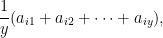$\displaystyle\frac{1}{y}(a_{i1}+a_{i2}+\cdots+a_{iy}),$ tồn tại 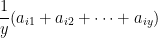$x$ số, chẳng hạn $\displaystyle\frac{1}{y}(a_{i1}+a_{i2}+\cdots+a_{iy})$ với $i=1,$ $2,\ldots,$ $x$ , có tổng chia hết cho $x.$ Khi đó $xy$ số $a_{ij}$ với $(i,j)\in [x]\times [y]$ có tổng chia hết cho $xy,$ suy ra khẳng định đúng với $xy.$

Vậy ta chỉ cần chứng minh nó đúng với các số nguyên tố. Giả sử $n=p$ là một số nguyên tố và $a_0,$ $a_1,\ldots,$ $a_{2p-2}$ là các số nguyên bất kỳ. Ta cần chỉ ra có $p$ số trong các số đã cho có tổng chia hết cho $p.$ Với mỗi số nguyên $\alpha,$ ký hiệu $(\alpha)_p$ là số dư khi chia $\alpha$ cho $p.$ Không mất tính tổng quát, giả sử $\{(a_i)_p\}$ là một dãy không giảm. Nếu tồn tại $i\in [p-1]$ sao cho $(a_i)_p=(a_{i+p-1})_p$ thì

$(a_i)_p=(a_{i+1})_p=\cdots =(a_{i+p-1})_p\Rightarrow \sum_{j=i}^{i+p-1}a_j\equiv 0\pmod{p},$ nếu không, xét $p-1$ tập $A_i=\{a_i,a_{i+p-1}\}$ và dùng hệ quả trong [1] ta có